Sequence of Return Risk By The Numbers

Sequence of return risk refers to the phenomenon by which a few bad years early in a retirement portfolio can cause havoc for the life of the portfolio. Sequence of return risk is only relevant if the portfolio amounts are changed by either an annual addition or withdrawal.

Consider the following annual returns:

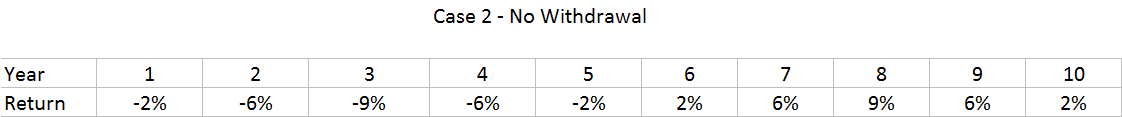
We begin with a portfolio worth $1 million and observe its value after 10 years. Note that Case 1 and Case 2 are the same five year returns just reversed.

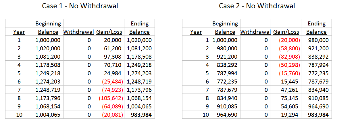
Both examples yield the same 983,984 ending balance. When a portfolio is untouched, sequence of return risk is not a concern.

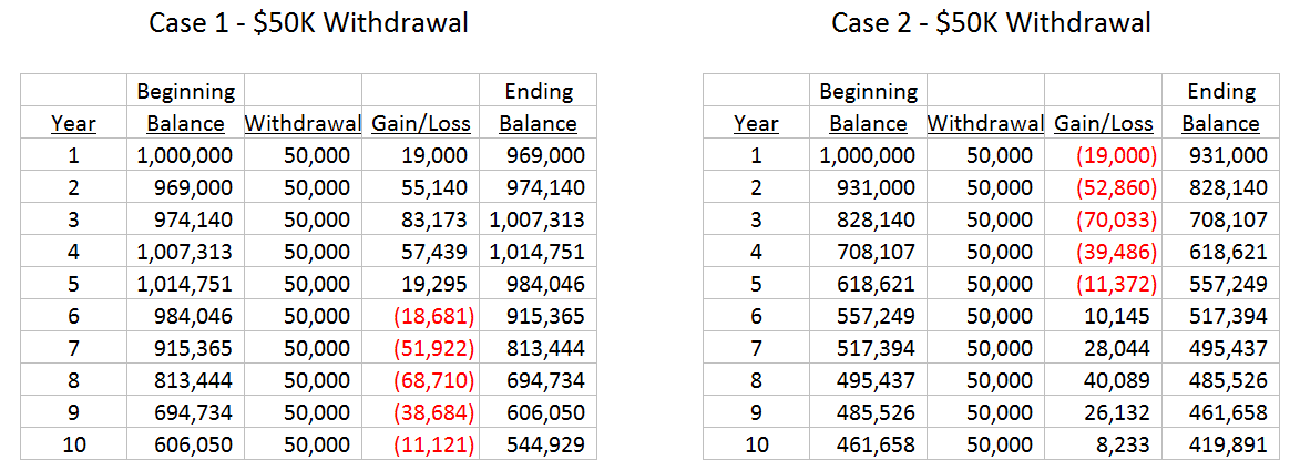
Unlike model portfolios, actual retirement portfolios realize periodic withdrawals.We revisit the Case 1 and Case 2 portfolio returns with an annual $50,000 withdrawal.We assume the withdrawals are made at the beginning of each year.This accounts for the differences in gains and losses.This time, the ending balances are substantially different.

Sequence of return risk is the evil twin of dollar cost averaging. When one invests in a portfolio through a dollar cost averaging program, one hopes that if the markets are going to have a rough patch, they do so early in the investment campaign. This gives the portfolio an opportunity to accumulate more shares early.

With sequence of return risk, the same math that offered an outstanding return in the case of a dollar cost averaging program, works against the investor/retiree. Negative early returns, coupled with annual withdrawals, compound the early declines resulting in a significant loss of portfolio valuation over time.In severe instances, early negative returns can remove any chance that a retirement portfolio can support a comfortable retirement.

Consider a longer time frame using actual market returns from two 30 year periods; 1988 through 2017 and 1926 through 1955. We obtained S&P 500’s annual returns courtesy of MoneyChimp.com.The website provides the S&P 500 returns with or without dividends and before and after accounting for inflation. For modeling purposes, we assume the S&P 500 as a proxy for market returns. Since we assume our retirement portfolio contains stocks and mutual funds (there were no ETF’s before 1993), we include dividends.

We assume the following for our portfolio.

• 60% equities, 40% bonds
• 30 years of S&P 500 returns for equities, bonds return 1.8% more than the average rate of inflation over the 30 year time period.
• Our portfolio has an initial value of $1 million
• Annual withdrawals begin at $52,500 (5.25% of the initial portfolio amount) and increase 3% annually.

We first consider a simple, noiseless example. Equities increase 8% annually while bonds increase 4.6% annually, just as we will find for the 1988 through 2017 timeframe.This is our perfect world scenario, unencumbered by market fluctuations.

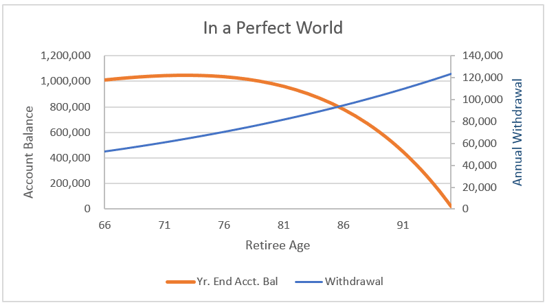
Base Case – 8% Equity, 4.6% Bond Annual Increases

At the end of 30 years, our portfolio is effectively exhausted.If our retiree began withdrawing the $52,500 at age 66, he/she is out of money at age 95. Our retiree has suffered no sequence of return risk as we assume a constant 8% annual return for equities and 4.6% return for debt.

We leave the perfect world of consistent returns to investigate two unique time periods; 1988 through 2007 and 1926 through 1955. For investors, the 1988-2007 period was outstanding. The 1926-1955 period was less robust. The annual S&P 500 returns for these periods, including dividends, are presented as follows:

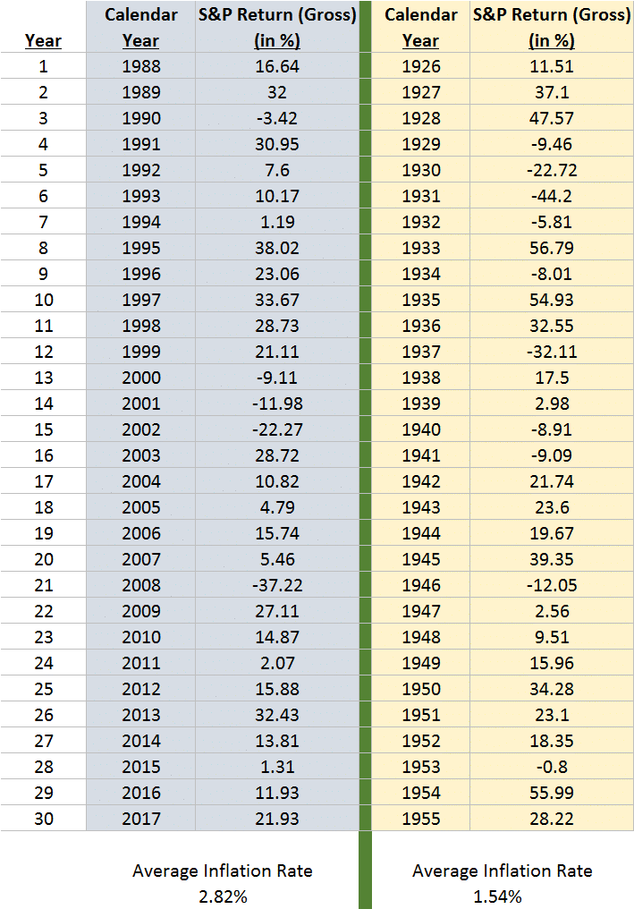
Ove the period 1988 through 2007, inflation averaged 2.8% over the period, so our bond portfolio pays 2.8% + 1.8% or 4.6%.

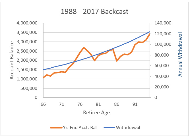
1988 Through 2007 – S&P500 Equity Returns, 4.6% Bond Returns w/ Rebalancing

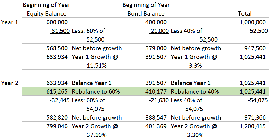
The computations for the first two years are presented below. Note the rebalancing (shown in green) beginning in Year 2 to maintain a 60/40 weighting.

Of the 30 years, S&P 500 returns were negative only 5 times with one year showing a minor 3.4% loss. Our graph shows that investors were well rewarded.

Our second time period included the Depression that began in 1929.Inflation over the period averaged 1.54%. We set our bond return at 1.8% more than inflation and round off to 3.3%. A retirement portfolio in existence from 1926 through 1955 did not fare nearly as well.

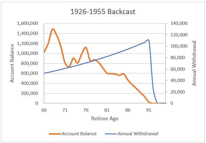
1926 Through 1955 – S&P 500 Equity Returns, 3.3% Bond Returns w/ Rebalancing

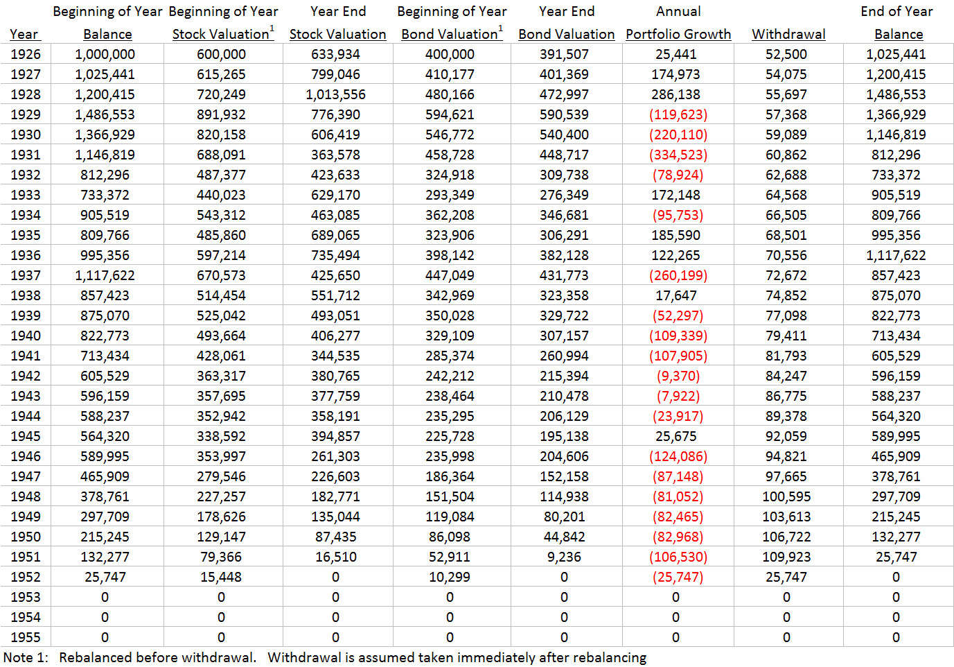
The math is the same as that employed in the previous time period.

Down years were only 9 out of 30, but their timing was front loaded. Sequence of return risk was responsible for significant damage to our portfolio depleting it of money after 27 years.

Rebalancing

Our 1988-2017 portfolio would have done well no matter what we did providing that we maintained a heavy equity exposure. By maintaining a 60% equity weighting, even the onset of the Great Recession in 2008 only cost us 20% of the total portfolio.

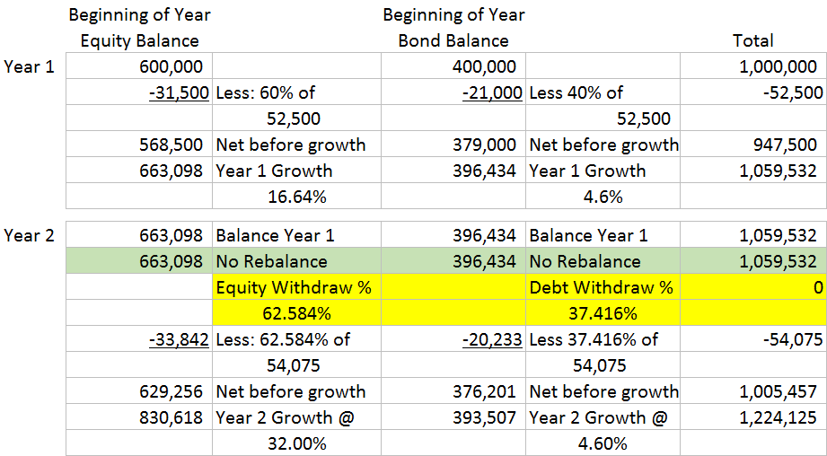
Financial experts tell us that asset allocation is the key to minimizing sequence of return risk in a portfolio’s long run return. In our previous examples, we reset our total funds to 60/40 equity to debt annually. What if we had not made this adjustment annually? We look at the numbers in a scenario where we split our annual withdrawal between equity and debt based on their relative portfolio sizes.We did not rebalance to 60/40 annually. What we found was that a failure to rebalance exacerbated the trends already in existence.

1988 Through 2007 – S&P 500 Equity Returns, 4.6% Bond Returns, No Rebalancing

The computations for the first two years are presented.Note that we do not rebalance (green). But we take an additional step to reweight the distributions. The two portfolios are no longer in a 60/40 balance. To avoid draining one of the accounts faster than the other, we determine the new weighting each year (shown in yellow).

The positive trend in place with rebalancing is now exaggerated by not rebalancing. The $3.4 million ending account balance has grown to $4.5 million.

Unfortunately, the multiplier effect is equally effective when the market returns are not favorable.

1926 Through 1955 – S&P 500 Equity Returns, 3.3% Bond Returns, No Rebalancing

The computations are as follows:

Our rebalanced portfolio was depleted in early 1952. Without rebalancing, our portfolio is depleted in early 1948, four years faster.

Conclusion

When one retires, the investment objective changes from growth to reducing variance. While working, there is always an opportunity to recoup losses. Time is on your side. A few bad years may actually provide a benefit if one is investing regularly and one has years to go before retirement.

In retirement the portfolio is set. Some equity exposure is necessary to realize gains well in excess of inflation. Too much exposure, however, makes the portfolio vulnerable to a few bad years. This is particularly true if the bad years come early in the portfolio’s life, a sequence of return risk incidence. There is no ability to reset a portfolio in retirement. If one is invested in equities, some losses are inevitable. It is critical to keep them manageable.

Rebalancing, also known as asset allocation, is the key to building a portfolio that will sustain a retirement with a high degree of confidence.Rebalancing keeps a portfolio from becoming overweight in any one asset class. Each asset class has its own mean long term annual return and variance.Asset classes are not perfectly correlated with each other. Regular rebalancing reduces a portfolio’s overall return variance making it less susceptible to sequence of return risk.